- Published on
Predicting timeseries data using Facebook Prophet in a Python Flask service, Influxdb and Grafana on Raspberry Pi
- Authors

- Name
- Peter Peerdeman
- @peterpeerdeman
As you have probably already noticed, I thoroughly enjoy collecting timeseries data using influxdb and grafana. With recent developments in AI gaining momentum, I was curious to see if I would be able to predict the future using my low-power home server setup.
Goal: predicting solar yield over the next year
I was already collecting and visualising solar panel data using influxdb, nodejs and pvoutput. This means we already have a timeseries database, there is a database present filled with a couple of years worth of energy generation measurements. Following this template, we could try to predict any influxdb timeseries! Before we get there, we need to take the following steps:
- Find the right timeseries prediction model
- Get prophet running on arm
- Turn Prophet into a REST API
- Query Influxdb data, make a prediction, store the results
- Visualise the predictions in Grafana
Researching timeseries prediction models
After some research, I found there are quite a number of methods to extrapolate timeseries data: Long Short-Term Memory (LSTM), Autoregressive Integrated Moving Average (ARIMA), SARIMA (ARIMA but with Seasons) and combinations of before: additive regression. I'm not getting into the super specifics here, if you are into that definitely read Krish Hariharan's blog on the theory behind these topics.
Making that easily accessible: Facebook Prophet
As I figured the project would already have enough going on with data flow and connecting different services, I decided to roll with Facebook's Prophet. Prophet uses the above techniques and exposes an easy to use datastructure and API so you can focus on getting your data in and predictions out, instead of applying the models yourself.
Trends, Yearly Seasonality, Weekly cycles
Prophet works best with with timeseries that have "seasonal" effects and a dataset that has several seasons worth of data. To get a basic idea of how Prophet works, check out this dataset with facebook data events:
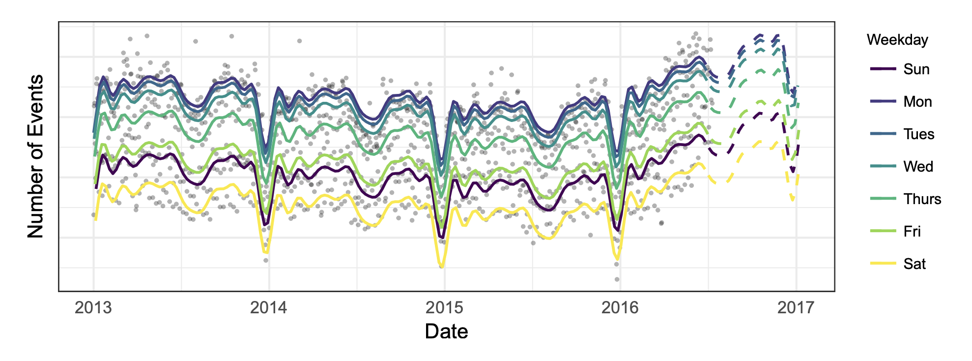
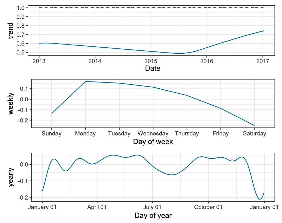
Prophet looks at a timeseries like this and tries to fit multiple graphs on top of eachother, in each using different cycles of time. A trendline over a longer period of time, a yearly cycle (e.g. with a dip in summer and december) and a weekly cycle (most activity on monday)
Now that we have an idea how the model works, let's setup that crystal ball and see if we can predict next years solar panel yield!
Let's go!
Getting Prophet running on Raspberry Pi ARM
My first step was to just get the prophet command even running on Raspberry PI's ARM architecture. I found this docker image by lppier that I could tweak to to get it running on arm:
- update the the python version
- explicitly use piwheels for the setuptools, cython dependencies
- omit use of slim image to make sure it builds
I could now build the image for arm using buildx, and get a first timeseries predictions on raspberry, using the example_wp_log_peyton_manning.csv example file!
» docker run -it peterpeerdeman/docker-prophet-arm:1.0.0-slim /bin/sh
# python app.py
Importing plotly failed. Interactive plots will not work.
Running https://facebook.github.io/prophet/docs/quick_start.html
           ds         y
0  2007-12-10  9.590761
1  2007-12-11  8.519590
2  2007-12-12  8.183677
3  2007-12-13  8.072467
4  2007-12-14  7.893572
INFO:fbprophet:Disabling daily seasonality. Run prophet with daily_seasonality=True to override this.
Initial log joint probability = -19.4685
    Iter      log prob        ||dx||      ||grad||       alpha      alpha0  # evals  Notes
      99       7975.09    0.00977601       175.243           1           1      129
    Iter      log prob        ||dx||      ||grad||       alpha      alpha0  # evals  Notes
     199       7993.41    0.00168694       471.644           1           1      253
    Iter      log prob        ||dx||      ||grad||       alpha      alpha0  # evals  Notes
     299       7998.48   0.000171241       168.202       0.599       0.599      372
    Iter      log prob        ||dx||      ||grad||       alpha      alpha0  # evals  Notes
     399       8000.49    0.00358088       328.878           1           1      489
    Iter      log prob        ||dx||      ||grad||       alpha      alpha0  # evals  Notes
     463       8001.24    7.5267e-05       159.116   8.492e-07       0.001      601  LS failed, Hessian reset
     499       8001.38   0.000122146       68.9352           1           1      652
    Iter      log prob        ||dx||      ||grad||       alpha      alpha0  # evals  Notes
     599        8002.8   8.58223e-05       150.448      0.7366      0.7366      769
    Iter      log prob        ||dx||      ||grad||       alpha      alpha0  # evals  Notes
     662       8003.41   0.000143616       240.605   1.255e-06       0.001      888  LS failed, Hessian reset
     699       8003.65   8.45692e-05       60.8838      0.4015           1      931
    Iter      log prob        ||dx||      ||grad||       alpha      alpha0  # evals  Notes
     774       8003.83   0.000152789       130.023    2.04e-06       0.001     1054  LS failed, Hessian reset
     799       8003.84    1.1178e-06       57.9922      0.2598           1     1090
    Iter      log prob        ||dx||      ||grad||       alpha      alpha0  # evals  Notes
     811       8003.84   1.24418e-05       56.1248   1.625e-07       0.001     1147  LS failed, Hessian reset
     819       8003.84   1.11276e-07       55.1786      0.0991      0.5314     1158
Optimization terminated normally:
  Convergence detected: relative gradient magnitude is below tolerance
             ds      yhat  yhat_lower  yhat_upper
3265 2017-01-15  8.215259    7.494644    8.870238
3266 2017-01-16  8.540339    7.780047    9.241987
3267 2017-01-17  8.327785    7.578004    9.060797
3268 2017-01-18  8.160444    7.412273    8.869641
3269 2017-01-19  8.172398    7.405505    8.856769
The app.py script is supplied with a csv file containing 2906 records of a date and a value, then predicts the following year of 356 values and prints the "tail" (last 5 values).
That's great and all, but 1) this is not our own home grown influx data yet, and 2) we cant see the resulting python graphs because we are running in docker. We'll build a realtime dashboard in grafana later, but lets first focus on the data.
Rasprophet: A Raspberry Prophet REST interface
Instead of running a command on our laptop when we want to make a prediction, I want to continually make new predictions and update the dashboard in near-realtime, so I don't have to wait for the prediction when I visit the dashboard. I figured we should start turning the prophet command into a generic service with a REST interface that we can keep querying.
Introducing Rasprophet, a small python application that is built on top of the above docker image, but uses a small Flask API to expose the Prophet functionality and allow us to use http to post data to the model.
The app defines an API that allows us to post timeseries data in a similar format as the example csv, and takes a parameter p that allows us to define how many prediction values s should be returned:
{
  "ds": [
    "2016-01-20",
    "2016-01-21"
  ],
  "y": [
    8.8999,
    9.9999
  ],
  "p": 2
}
We can now run the Rasprophet service using docker and make our first request using curl:
docker run -it --rm -v "$PWD":/app -p 5000:5000 peterpeerdeman/rasprophet-prophet-rest-service:1.0.0
curl -X POST --header "Content-Type: application/json" --data '{"ds":["2016-01-20","2016-01-21"],"y":[8.8999,9.9999],"p":2}' localhost:5000 | jq
» curl -X POST --header "Content-Type: application/json" --data '{"ds":["2016-01-20","2016-01-21"],"y":[8.8999,9.9999],"p":2}' localhost:5000 | jq
  % Total    % Received % Xferd  Average Speed   Time    Time     Time  Current
                                 Dload  Upload   Total   Spent    Left  Speed
100  1011  100   951  100    60   1160     73 --:--:-- --:--:-- --:--:--  1232
{
  "additive_terms": {
    "2": 20.48951864573794,
    "3": 31.64524628648716
  },
  "additive_terms_lower": {
    "2": 20.48951864573794,
    "3": 31.64524628648716
  },
  "additive_terms_upper": {
    "2": 20.48951864573794,
    "3": 31.64524628648716
  },
  "ds": {
    "2": "Fri, 22 Jan 2016 00:00:00 GMT",
    "3": "Sat, 23 Jan 2016 00:00:00 GMT"
  },
  "multiplicative_terms": {
    "2": 0.0,
    "3": 0.0
  },
  "multiplicative_terms_lower": {
    "2": 0.0,
    "3": 0.0
  },
  "multiplicative_terms_upper": {
    "2": 0.0,
    "3": 0.0
  },
  "trend": {
    "2": -8.934402385980752,
    "3": -18.231002061023013
  },
  "trend_lower": {
    "2": -8.934402467119432,
    "3": -18.231002322794264
  },
  "trend_upper": {
    "2": -8.934402310405922,
    "3": -18.231001832176318
  },
  "yearly": {
    "2": 20.48951864573794,
    "3": 31.64524628648716
  },
  "yearly_lower": {
    "2": 20.48951864573794,
    "3": 31.64524628648716
  },
  "yearly_upper": {
    "2": 20.48951864573794,
    "3": 31.64524628648716
  },
  "yhat": {
    "2": 11.55511625975719,
    "3": 13.414244225464149
  },
  "yhat_lower": {
    "2": 11.55511617809335,
    "3": 13.414243961756155
  },
  "yhat_upper": {
    "2": 11.55511633548562,
    "3": 13.414244451248319
  }
}
Gluing the services together with Node
Again, great but it is still not realtime influxdb data. To glue our services together I've created an "influx-to-prophet" nodejs script that:
- queries influxdb for the pv data
- transforms that data into json that rasprophet can work with
- send the formatted data to the rasprophet API endpoint
- parse the results, prepare them for influxdb
- store the results in influxdb
we can modify the script to use the correct influxdb url and measurement query, run this script using node influx-to-prophet-workinprogress.js and we could even schedule it to let it run every x seconds.
We are very close now, as the prediction data is now getting stored into influx: we just need to visualise it. Hello grafana!
Visualise predictions using grafana
Back in grafana we can now create a panel and fill the query for the original pv power generation:
SELECT mean("powerGeneration") FROM "pvstatus" WHERE $timeFilter GROUP BY time(3d) fill(previous)
If we now add a second, third and fourth query we can now query the prediction data: a prediction, a prediction lower value and the prediction higher value from the pvstatus_predictions that was created with the nodejs gluecode. I've added the "prophetprediction" tag so you could even write the measurement into the same measurement you got the data from and still select it:
SELECT mean("yhat") FROM "pvstatus_predictions" WHERE ("origin" = 'prophetprediction') AND $timeFilter GROUP BY time($__interval) fill(previous)
SELECT mean("yhat_lower") FROM "pvstatus_predictions" WHERE ("origin" = 'prophetprediction') AND $timeFilter GROUP BY time($__interval) fill(previous)
SELECT mean("yhat_upper") FROM "pvstatus_predictions" WHERE ("origin" = 'prophetprediction') AND $timeFilter GROUP BY time($__interval) fill(previous)
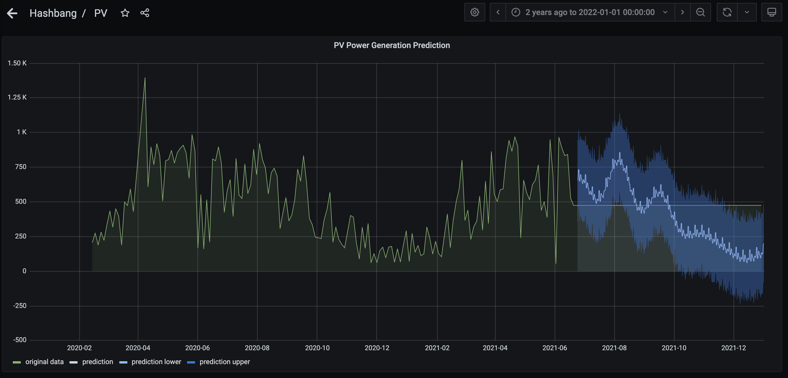
If you now go to the options pane on the right, go to "series overrides" and create one override for prediction lower and one for prediction upper with "fill below to: prediction lower" setting, you can see your brand new prediction in the same graph as the original data:
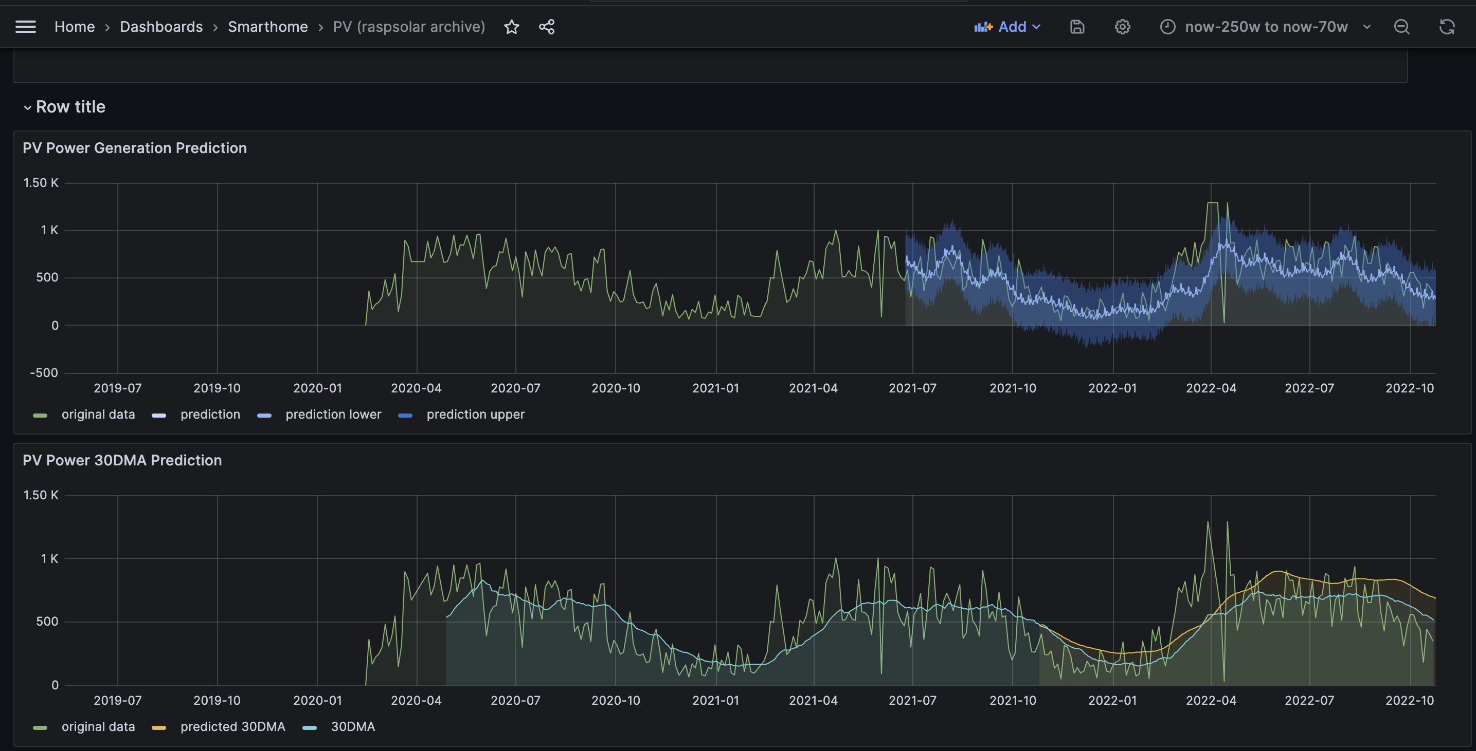
It was quite fun to see that the seasonality was quite well predicted, especially if you take 30 day moving average values from the data. I've added a screenshot of this blog 10 months later to compare the predictions back then to the actual values:
As next steps, I'm looking forward to investigating a robust MLOps solutions such as kubeflow or Argo to schedule these workloads and recurring jobs reliably.
check out the other blogs on the timeseries and forecasting topic here:
- Using influxdb, grafana and nodejs datalogger rasplogger to visualise solar panel data
- Using Darts-Timeseries-Forecaster to perform configurable forecasting on timeseries
- Continuous forecasting with MLops pipeline on Kubernetes using Argo workflows, Influx and Darts
Edit: blog updated 2024-02